Objectives for Data Collection Missions:

Collect high quality photos with sufficient metadata and supporting ground information to build effective orthomosaics and terrain models that will inform downstream analyses.

General Photo Capture Guidelines:

UAS acquired photos – both RGB and multispectral – must be properly exposed, non-blurry with good contrast, be geotagged (very strongly encouraged, but not critical if high quality GCP available).  Examine images for motion blur or exposure issues immediately after flight.  Avoid days when there are changing cloud conditions during flight, as this will affect spectral properties and the mosaicking process.  Shoot in RAW+jpeg or TIFF when possible, but if you are only able to use jpeg, be consistent with white balance settings across all flights.  Make sure your camera’s time and date is properly set and remains accurate throughout different flight periods. Clearly note if this is local time or UTC (what GPS uses). These time and date records will be stored in the .EXIF files associated with your images and can be of great archival value.

Gather pre and post flight photos of calibration targets (in addition to in flight targets if available) for each mission to allow for better radiometric correction and cross site comparisons. These comparisons will be of less value for some cameras (especially consumer RGB) than others, but consistent methods here will provide insights for future protocols and will be of value for downstream analyses.  Calibration Protocols and guides: HiLDEN: Spectral Calibration and Guidance and Additional Information on Pre-/post-flight Calibration Targets.

Multi-scale tundra mapping for structural and spectral data:   

At each tundra block, teams should map nested plot samples stratified by altitude (detailed below) during the peak of the growing season (priority) and other times when time and resources are available (i.e. vegetation emergence period, mid-greenup, senescence). This should be done for both RGB and Multispectral sensors (if available).

We chose standardized flight altitudes for 2017 rather than standard ground sampling distance (GSD, i.e. pixel size) to simplify protocols for the data collection this summer. To be clear, we will not be directly comparing multispectral data (often much coarser native grain at given altitude) from one site to RGB data (often might finer native grain) at another site. Instead, where both Multispectral and RGB data are available, we will pair them with each other to generate synthesis products. Furthermore, as most groups do not have terrain-tracking capabilities in their flight planning this summer, actual GSD will vary in part as a function of terrain. The variability in GSD among common high-res (~15-20 megapixel) RGB sensors flown at given altitudes will be relatively small (1-3cm difference) and will dealt with analytically.

We ask that teams fly a sample of each tundra block at four flight altitudes (so 4 RGB and/or 4 multispectral if available) detailed in the list and figure below:

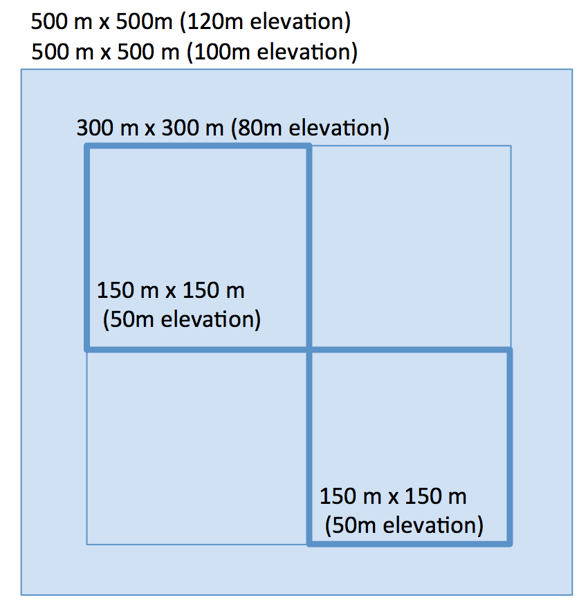
• 500 x 500m @ 120m altitude
• 500 x 500m @ 100m altitude
• 300 x 300m @ 80m altitude
• 150 x 150m @ 50m altitude (2 plots)

In sum, this hierarchy of flights and sensors at a given blocks is equivalent to one ‘block’ replicate. We would like a minimum of three block replicates per field site.  In the figure above we have nested two 50m flights within the 80m flight level box.  When choosing specific layout for nested plots, avoid putting smaller plots alongside edges of the larger tundra block to reduce the impact of edge artifacts that often arise during model construction on downstream analyses.

We ask that you fly these missions at our around the timing of peak vegetation productivity (generally towards the end of July or first week of August at most tundra sites).  This will allow for standardized comparisons across sites.  If time and resources allow, you are welcome to contribute data from outside of peak season as well, as some teams will also be gathering time-series for phenological monitoring, though this is not a primary focus for the 2017 cross-site analysis (if enough teams are interested, however, we can also focus on this too!).  If you are not in the field during peak season, fly at a date during the green-up period.  Other particular time periods of interest are just prior to/during onset of growing season or during senescence.

Note: Most projects are using multi-rotor drones, and some are using both fixed-wing and multi-rotor units. If you ONLY have a fixed wing unit, it is unlikely you will be able effectively gather data at 50m or perhaps even 80m in some environments. In these cases, skipping lower-altitude data collection is completely understandable – please do not try to do anything unsafe/beyond the capabilities of your platform or out with the local regulations for flight altitudes or other flight parameters.

Mission Planning Background:

There are a variety of software ‘apps’ or programs that enable systematic flight planning and image capture.  This is preferable to manual/semi-manual flights over the mapping areas for repeatability, analytical, and safety reasons. If you have a software system you prefer, feel free to utilize that as long as you are able to: a.) keep consistent records of flight plans, and b.) it is capable of creating flights resulting in proper image overlap/quality. If you are unable to meet this requirements, please keep as detailed records as possible with points a.) and b.) in mind.

Suggested mission planning apps:

• For Pixhawk/3DR systems – Mission Planner (available only on PC)
• For DJI systems – DJI GS PRO (http://www.dji.com/ground-station-pro), other available apps include Pix4D Capture (https://pix4d.com/product/pix4dcapture/), Altizure (https://www.altizure.com/), DroneDeploy (https://www.dronedeploy.com/), etc. but not all of these apps can currently provide the same functionality as DJI GS PRO.

 

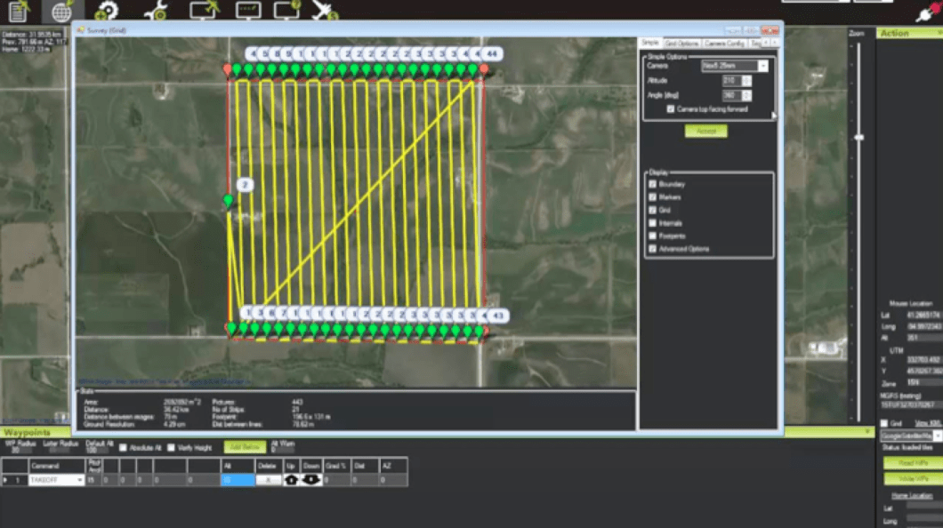
Each of these apps will be able to generate a lawnmower-style (like this screenshot from Mission Planner below) or cross-gridded flight path.  These plans result in several overflights of the same area with automated camera triggering to generate desired image overlap.  The combination of app, airframe, and camera will differ for each working group and site.  There are several excellent tutorials on YouTube and elsewhere online that can be used to go over the specific details of these hardware/software pairings for less experienced pilots.  We can also offer specific advice – particularly for MissionPlanner, DJI GS PRO and Altizure systems upon request (jtkerb@gmail.com).  Ultimately, there are many systems that can produce high quality data, but regardless of system, special care needs to be taken by all contributors to ensure data meet the shared mission planning objectives listed below that are designed to allow for consistent comparisons across sites and through time.

Mission Planning Protocols for HiLDEN:

When planning missions, have mission plans extend 20m beyond the desired mapping area.  The edges of orthomosiacs are prone to stitching errors due to reduced image overlap in these regions, especially if they are located upslope from the takeoff location.  For most flights, you will want to fly with the cameras facing nadir, i.e. directly downward, although for some structural models you may want additional flights with the camera at a slightly oblique angle (specific angle off nadir will depend on environment, start with 20 degrees).  If your drone tilts at a predictable angle while in motion and you are using a static camera mount, try to adjust for this selecting the angle you mount the camera at when planning for nadir images.

Image overlap is critical for building structural models and orthomosaics. There are different ways to optimize data collection for these builds to address specific questions, but many include planning for specific environments go beyond the level of detail of a general protocol and HiLDEN questions. For the cross field-site analysis, we ask groups to plan for missions that have >20 overlapping images for any given point being mapped. This can be achieved via adjusting the sidelap, forelap, and number of mission overflights for a given area. For example: 66% sidelap and 80% forelap should yield ca. 15 photos per location, whereas 66% sidelap and 90% forelap should yield ca. 30 photos per location. 95% sidelap and 33% forelap should also yield ca. 30 photos per location, but might be a more attainable combination for particular hardware configurations (e.g. low trigger rate camera on a fixed wing).

If you are unable to work out these specific calculations, a safe bet is to aim for at least 80% front and 80% sidelap in their images, a concept illustrated below from a graphic from DroneDeploy.  This combination of overlap creates multiple images of a given area, even over varying terrain.  Some drone companies/software programs suggest lower overlapping values for image capture. This is a reflection of them thinking about the analytical stage of processing assuming perfect data collection with no error between mission plan and real world data acquisition. Error propagates during structural builds as a function of the angle that overlapping images are acquired from (this is optimized around 65% overlap at about 100m). However, this perspective does not factor in real-world flying conditions! The consequences of having too little overlap (due to drone mission being affected by wind or varying terrain) are much more impactful on model output (i.e. model failure!) than having too much overlap (increased noise to signal ratio in structural builds – however, this can also be addressed in post-processing using filtering algorithms). These insights reflect field experiences from many research teams.

If you are unable to program in overlap parameters into your mission plan (first try another program!), then you may want to set your camera’s interval timer to the shortest interval setting that it allows for continual image capture (i.e. somewhere around every 2 seconds).  Calculating image footprint and grain sizes to address these problems manually can be done via simple geometry with camera and flight inputs.  A spreadsheet template for this approach can be found here (from Pix4D):

https://s3.amazonaws.com/mics.pix4d.com/KB/documents/Pix4D_GSD_Calculator.xlsx

When planning the flight speed of your missions, you need to balance tradeoffs between faster speed to cover a large area and slower speed to generate higher quality images.  This tradeoff varies with flight and camera specifics, so a little bit of trial and error is required to find the optimum where photos are of high quality and you are able to cover the desired extent.  Some extents will require two or more flights to cover the entire flight area depending on the hardware being used. As noted earlier, it is unlikely a fixed wing will be able to flow slow enough to capture data at 50m, or in some cases, even 80m.

Ground Control and Truthing for Synthesis Paper

Building high-fidelity structural models and orthomosaics benefits from having information on camera location, and is best constrained by ground control markers.  A thorough review of this process and its optimization is forthcoming, but by following the procedures below, these protocols will be standardized across sites.

Ground Control Markers:

As mentioned in previous posts, ground control markers should be readily visible from the air, stand out in all spectral bands being captured, and be immobile during the flight period.  Ideally the center of these ground control markers should be geolocated using a differential Global Navigation Satellite System (dGNSS) like a dGPS down to a few centimeters. Place approximately 20 markers within each 500m x 500m block, with at least 6 of them in the smallest 150m x 150m sample areas.  Try to spread them evenly throughout the extent and associate each with a unique ID.  Consider placing permanent markers in some areas if you will return in future years, even if it is a smaller marker than can be used to re-place a larger marker in the future.  Also consider taking high-accuracy dGNSS location points at clearly defined edges/landmarks of naturally occurring (non-mobile) features (e.g., large rocks, ponds, etc.).  A good place for GCP is also the corner markers of your plots.

If no dGNSS system is available, we will most likely use the camera geolocation data as the primary source of spatial constraint during model builds. That said, it is still valuable to place GCP that are marked with traditional GNSS (e.g. GPS) in case .EXIF photo geolocation data are lost/corrupted. If no dGNSS is available, place GCP in clusters ~10 to 50m apart from each other. Assign a GPS location to each, and carefully measure the distances between these GCPs using a field measuring tape and/or laser range finder (and record these distances). You can even use your drone’s GPS to mark points! The GPS locations will be used as reference to visually locate these GCP in the final ortho, and the model can then be accurately scaled/validated using these distance measurements (in lieu of dGNSS points). Aim for four of these GCP clusters (of 3 – 4 GCP) in these situations.

Landcover Ground Truthing Data Collection:

For each tundra block, teams should write a descriptive statement about the types and form of vegetation in the landscape and provide any general information known about site history.  Please include photographs of dominant vegetation species as seen from the ground, and include an annotated (for example via powerpoint) sample of 4 – 6 drone photographs that identify these species and phenophase from above (example below from 120m altitude flight) and any signs of disturbance, herbivore presence, or anything you think is noteworthy.

Furthermore, teams should collect canopy height measurements from 30 or more locations within each block stratified across land-cover types and locations.  Associate these height records with a GNSS (i.e. GPS) record and/or with a point identified in a drone image (for example, like those above).

Selected Examples:

1. Betula nana, leaves out
2. Cerastium alpina, mature, a few flowers in wet area
3. Salix glauca, leaf buds opening, some leaves out
4. Tussock field, mostly Eriophorum sp. and Festuca sp.
5. Exposed rock in wind eroded area.

Also visible: trails used by caribou & researchers, etc…

Reminders to check before capturing image data:

• Geotagging is enabled
• Camera Date/Time are accurate
• Front and side overlap for images in mission plan is >80%
• RAW+jpeg capture is turned on
• Try to use (camera limitations and conditions  may require adjustments):
  • Fixed aperture
  • Fast shutter speeds (1/1000 or faster)
  • Low ISO of around 200 or less
• Fly slower the lower you are to the ground (to avoid image blur)